1. How to mount the probe - SCN-500 series
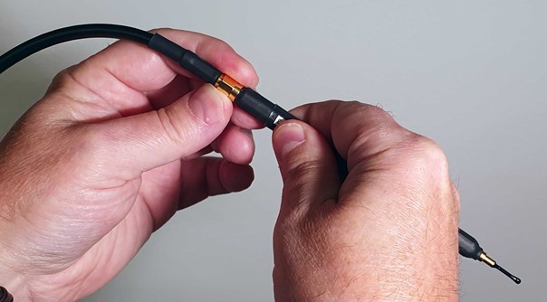
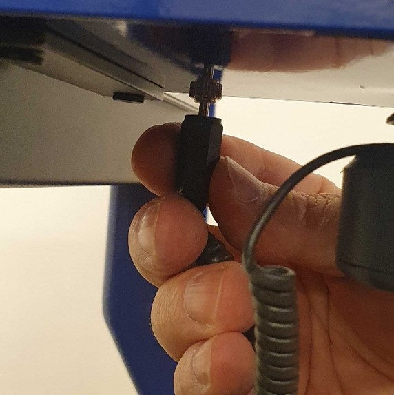
Connect the RF cable to the probe and tighten the nut firmly. It is very important that the nut is firmly tighten because of the rotation forces that will occur during four axis measurements.
Insert the probe from the top of the Z axis.
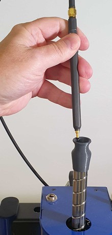
Fasten the probe by tightening the nut firmly.
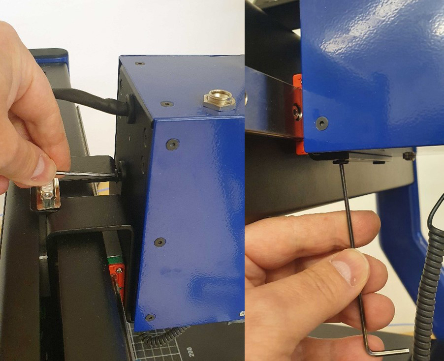
2. How to mount the ZR module - SCN-500 series
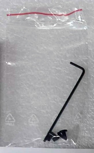
In the package with the SCN-500 EMC Scanner there is a small plastic bag with three screws and an Allen key. Those are for mounting the ZR module.
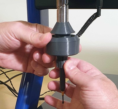
Mount the ZR module and fasten it with the upper screw first. Then fasten the two screws a the bottom.
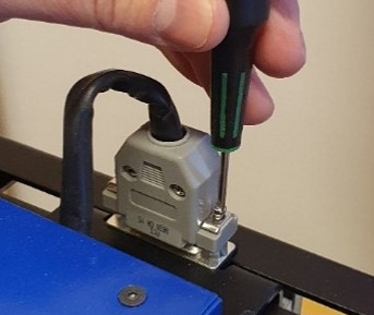
Connect the 15-pin D-SUB and secure it with the two screws. Use a regular flat head screwdriver.
Connect the probe holder to the ZR module.
3. How to perform Pre-Scan and EMC-Scan measurements
This chapter will guide you through, step by step, how to perform a simple EMC-Scan measurement step by step.
1. Start the software by clicking on the icon on your desktop.

2. After a few seconds, this dialog box will show.
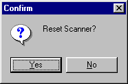
3. Click on Yes to reset the Scanner to its starting.
4. Position and calibrate the near field probe according to the procedure in “Positional calibrating the near field probe”.
5. Make sure that the near field probe is connected to the spectrum analyzer (possibly via a pre-amplifier) and that all instruments are powered on.
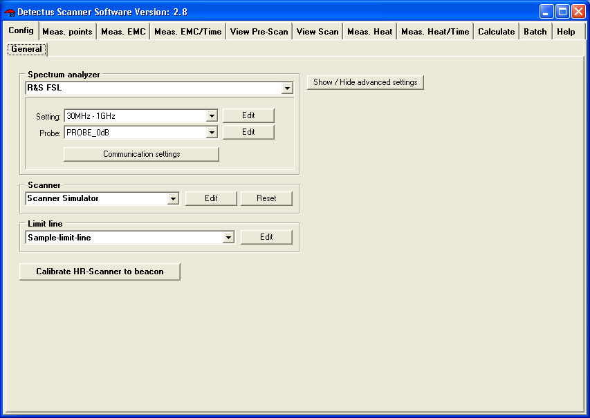
6. Click on the Config tab.
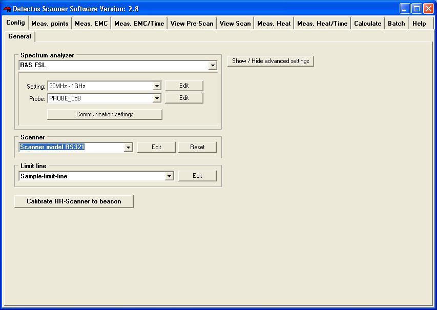
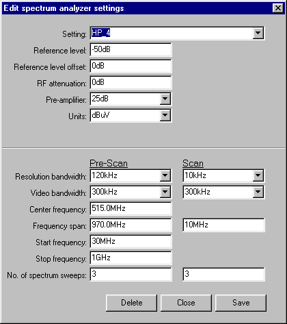
7. In the Spectrum analyzer box, near Setting, click on the Edit button. This is the Settings dialog box.
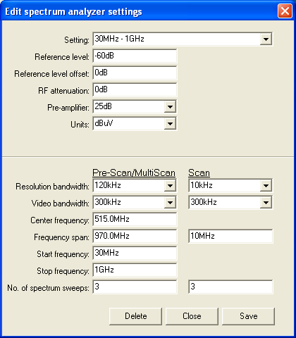
8. Click on the ”down arrow” on the right side of the Setting box and select a suitable setting from the list showing all stored settings. If no suitable setting is found, you may enter a new setting name and alter the settings to suit.
9. Click on the Save button.
10. Click on the Close button.
11. Click on the Config tab.
In the Spectrum analyzer box, near the Probe setting, click on the Edit button.
12. Click on the ”down arrow” on the right side of the Probe box and select a suitable setting from the list showing all stored settings. If no suitable setting is found, you may enter a new setting name and alter the settings to suit. (Refer to “Entering the amplitude correction factors of the near field probe”).
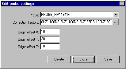
13. Click on the Save button.
14. Click on the Close button.
15. Place the test object on the Scanner table.
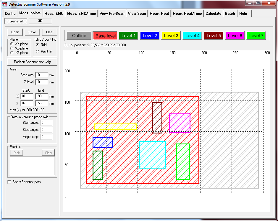
16. Click on the Meas. points tab.
17. Click on the General button to select 2.5 dimensional measuring points. It is also possible to generate full 3D measuring points. See “How to generate 3D measuring points” for a detailed description.
18. In the Grid / Point list box, select Grid.
19. Enter a suitable step size in the Step size box.
A small step size will generate a high-resolution measurement and a large step size will generate a low-resolution measurement.
Measuring in large steps is quicker than measuring in small steps.
20. Select measuring plane by clicking on XY plane, XZ plane or YZ plane.
21. Click on the Outline button.
Define the outline of the test object by entering values in the Area box. You may also click and draw the outline. Drawing the outline is optional, but may be valuable when you want to repeat a measurement.
22. Click on the Base level button.
Define the measuring area by entering values in the Area box. You may also click and draw the area.
23. Enter the value of Z-level in the Area box.
Z- level is the height of the probe above the Scanner table during measurement.
24. You may define “islands” with different Z-levels than the Base level by clicking on Level 1 … Level 7 buttons. This is useful e. g. to make the probe skip over high components on a PCB.
25. The measuring point can be saved (as an .MP file) for later use by clicking on the Save button.
26. Click on the Meas. EMC tab
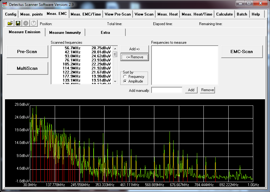
27. Click on the Pre-Scan button to start the wide-band measurement. (The setting for this measurement was defined in step 6.)
When the measurement is finished, you will see the spectra and a list of peaks.
28. Click on the Save button to save the measurement.
(Saving is optional, but you will find it useful when you want to repeat a measurement and compare the results.)
29. Select the desired frequencies from the list of Scanned frequencies and click on the Add => button to move the frequencies into the list of Frequencies to measure.
Other ways of entering a frequency into the list of Frequencies to measure, are by double-clicking on the spectra graph or simply by typing the frequency into the Add manually box and clicking on the Add button next to it.
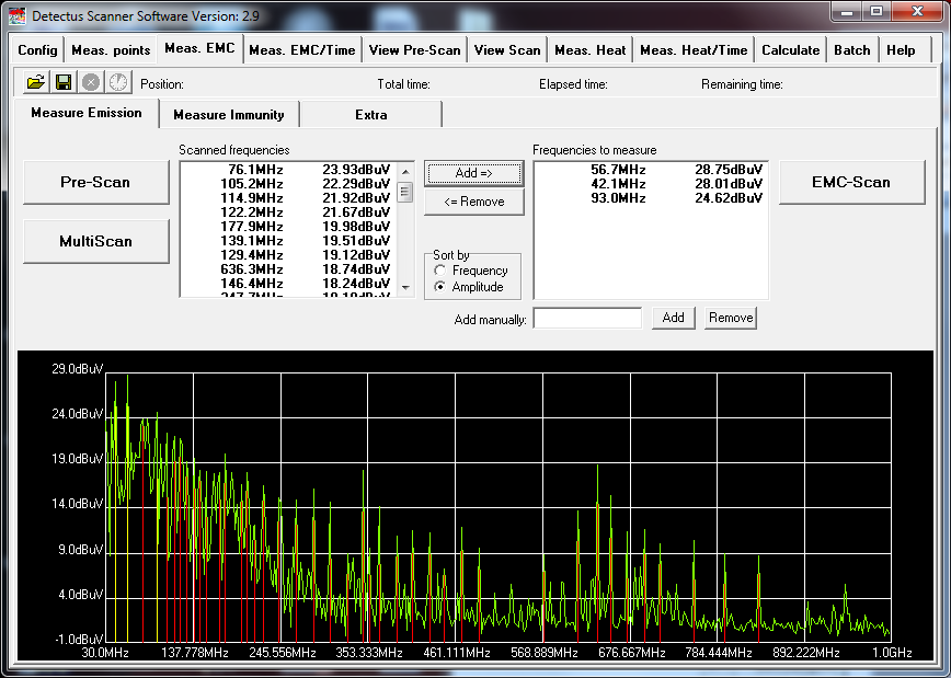
30. Click on the EMC-Scan button to start the narrow-band measurement of the selected frequencies. (The setting for this measurement was defined in step 6.)
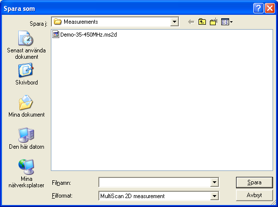
31. Before the measurement is started, you will have to enter where to save the result as one or more files.
32. Enter the desired file name.
You do not have to enter the file extension because the files will automatically be named .E01 for the first frequency, .E02 for the second frequency and so on. The measuring results stored in these files can be visualized on the View Scan tab.
33. Click on the View Scan tab.

34. There are many ways to visualize the result of an EMC-Scan measurement, utilizing the features on the View Scan tab. For detailed information, please refer to page 131.
35. The result of an EMC-Scan measurement can be documented as a report in HTML format and printed out.

4. How to perform a Multi-Scan measurement
This chapter will guide you through, step by step, how to perform a simple EMC-Scan measurement step by step.
1. Start the software by clicking on the icon on your desktop.
2. After a few seconds, this dialog box will show.
3. Click on Yes to reset the Scanner to its starting position.
4. Position and calibrate the near field probe according to the procedure in “Positional calibrating the near field probe”.
5. Make sure that the near field probe is connected to the spectrum analyzer (possibly via a pre-amplifier) and that all instruments are powered on.
6. Click on the Config tab.

7. In the Spectrum analyzer box, near Setting, click on the Edit button. This is the Settings dialog box.
8. Click on the ”down arrow” on the right side of the Setting box and select a suitable setting from the list showing all stored settings. If no suitable setting is found, you may enter a new setting name and alter the settings.
9. Click on the Save button.
10. Click on the Close button.
11. Click on the Config tab.
In the Spectrum analyzer box, near the Probe setting, click on the Edit button.

12. Click on the ”down arrow” on the right side of the Probe box and select a suitable setting from the list showing all stored settings. If no suitable setting is found, you may enter a new setting name and alter the settings to suit. (Refer to “Entering the amplitude correction factors of the near field probe”).
13. Click on the Save button.
14. Click on the Close button.
15. Place the test object on the Scanner table.
16. Click on the Meas. points tab.
17. Click on the General button to select 2.5 dimensional measuring points. It is also possible to generate full 3D measuring points. See “How to generate 3D measuring points” for a detailed description.
18. In the Grid / Point list box, select Grid.
19. Enter a suitable step size in the Step size box.
A small step size will generate a high-resolution measurement and a large step size will generate a low-resolution measurement.
Measuring in large steps is quicker than measuring in small steps.
20. Select measuring plane by clicking on XY plane, XZ plane or YZ plane.
21. Click on the Outline button.
Define the outline of the test object by entering values in the Area box. You may also click and draw the outline. Drawing the outline is optional, but may be valuable when you want to repeat a measurement.
22. Click on the Base level button.
Define the measuring area by entering values in the Area box. You may also click and draw the area.
23. Enter the value of Z-level in the Area box.
Z- level is the height of the probe above the Scanner table during measurement.
24. You may define “islands” with different Z-levels than the Base level by clicking on Level 1 … Level 4 buttons. This is useful e. g. to make the probe skip over high components on a PCB.
25. The measuring point can be saved (as an .MP file) for later use by clicking on the Save button.
26. Click on the Meas. EMC tab
27. Click on the Multi-Scan button to start the wide-band measurement. (The setting for this measurement was defined in step 7.)
Before the measurement is started, you will have to enter the location to save the result as one or more files.
28. Enter the desired file name.
You do not have to enter the file extension because the files will automatically be named .MS2D. The measuring results stored in this file can be visualized on the View Scan tab
29. Click on the View Scan tab.
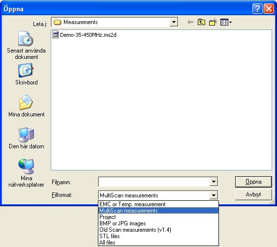
30. Change the search criteria at the bottom in the format box so that you can see the Multi-Scan files.
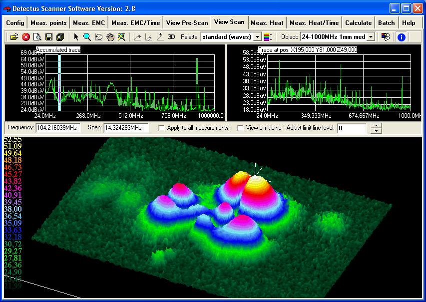
31. There are many ways to visualize the result of a Multi-Scan measurement by utilizing the features on the View Scan tab. For detailed information, please refer to page 131.
32. The result of an Multi-Scan measurement can be documented as a report in HTML format and printed out.
5. How to perform a Heat-Scan measurement (DS and Rx series)
This chapter will guide you, step by step, through a simple Heat-Scan measurement step by step.
1. Start the software by clicking on the icon on your desktop.
2. After a few seconds this dialog box will show.
3. Click on Yes to reset the Scanner to its starting position at coordinates X0 Y0 Z10.
4. Position and calibrate the IR-probe according to the procedure in “Positional calibration of the IR-probe against Scanner”.
5. Click on the Meas. points tab.
6. Click on the General button to select 2.5 dimensional measuring points. It is also possible to generate full 3D measuring points. See “How to generate 3D measuring points” for a detailed description.
7. In the Grid / Point list box, select Grid.
8. Enter a suitable step size into the Step size box.
A small step size will generate a high-resolution measurement and a large step size will generate a low-resolution measurement.
Measuring in large steps is quicker than measuring in small steps.
9. Select the desired measuring plane by clicking on XY plane, XZ plane or YZ plane.
10. Click on the Outline button.
Define the outline of the test object by entering values into the Area box. You may also click and draw the outline. Drawing the outline is optional, but you will find it useful when you want to repeat a measurement.
11. Click on the Base level button.
Define the measuring area by entering values into the Area box. You may also click and draw the area.
12. Enter the value of Z-level into the Area box.
Z- level is the height of the probe above the Scanner table during measurement.
13. You may define “islands” with different Z-levels than the Base level, by clicking on the Level 1 … Level 4 buttons. This is useful e.g. to make the probe skip over high components on a PCB.
14. The measuring points can be saved (as .MP files) for later use by clicking on the Save button.
15. Click on the Meas. Heat tab.
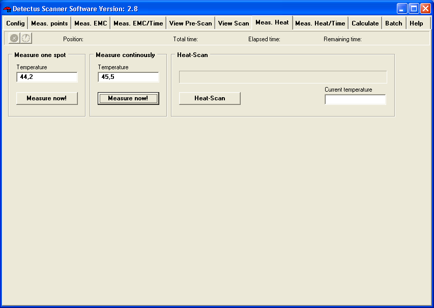
16. Click on the Heat-Scan button to start the measurement.
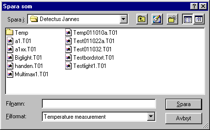
17. Before the measurement is started, you will have to enter the location to save the result file.

18. Enter the desired file name.
You do not have to enter the file extension because the file will automatically be named .T01. The measuring results stored in these files can be visualized on the View Scan tab.
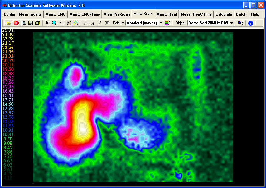
19. Click on the View Scan tab.
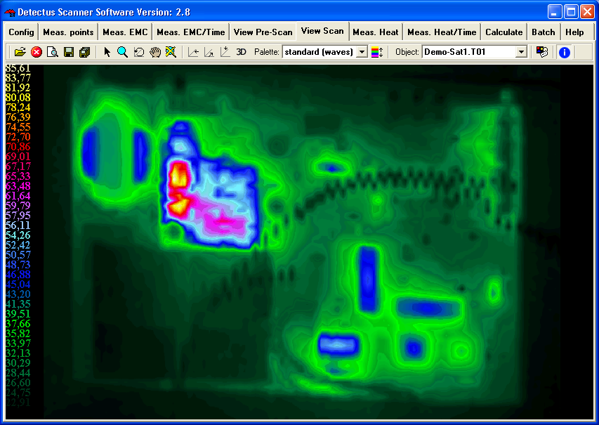
20. There are many ways to visualize the result of a Heat-Scan measurement by utilizing the features on the View Scan tab. For detailed information, please refer to page 131.
21. The result of a Heat-Scan measurement can be documented as a report in HTML format and printed out.
6. How to perform a Pre-Scan measurement on specified positions (DS and Rx series)
This chapter will guide you step by step through a Pre-Scan measurement on specified positions.
1. Start the software by clicking on the icon on your desktop.
2. After a few seconds this dialog box will show.
3. Click on Yes to reset the Scanner to its starting position at coordinates X0 Y0 Z10.
4. Position and calibrate the near field probe according to the procedure in “Positional calibration of the near field probe”.
5. Make sure that the near field probe is connected to the spectrum analyzer (possibly via a pre-amplifier) and that all instruments are powered on.
6. Click on the Config tab.
In the Spectrum analyzer box, near Setting, click on the Edit button.
7. Click on the ”down arrow” on the right side of the Setting box and select a suitable setting from the list showing all stored settings. If no suitable setting is found, you may enter a new setting name and alter the settings.
8. Click on the Save button.
9. Click on the Close button.
10. Click on the Config tab.
In the Spectrum analyzer box, near the Probe setting, click on the Edit button.

11. Click on the ”down arrow” on the right side of the Probe box and select a suitable setting from the list showing all stored settings. If no suitable setting is found, you may enter a new setting name and alter the settings to suit you. (Refer to “Entering the amplitude correction factors of the near field probe”).
12. Click on the Save button.
13. Click on the Close button.
14. Place the test object on the Scanner table.
15. Click on the Meas. points tab.
16. Click on the General button to select 2.5 dimensional measuring points. It is also possible to generate full 3D measuring points. See “How to generate 3D measuring points” for a detailed description.
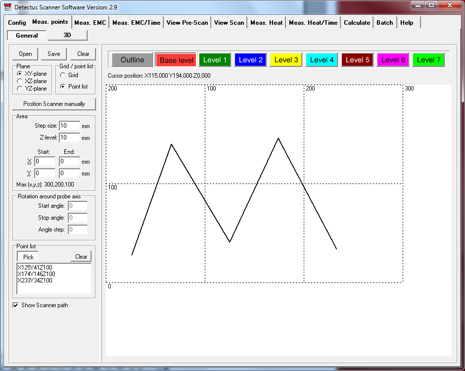
17. In the Grid / Point list box, select Point list.
18. In the Point list box, click on the Pick button.
19. Pick a desired number of points by clicking on the grid.
A dialog box will ask you to enter the Z-level of each point.
20. The measuring points can be saved (as .MP files) for later use by clicking on the Save button.
21. Click on the Meas. EMC tab.

22. Click on the Pre-Scan button to start the wide-band measurement.
(The setting for this measurement was defined in step 6. When the measurement is finished the spectra graph and a list of peaks are displayed.
23. Click on the Save button to save the measurement as a .PRE file.
24. Click on the View Pre-Scan tab.
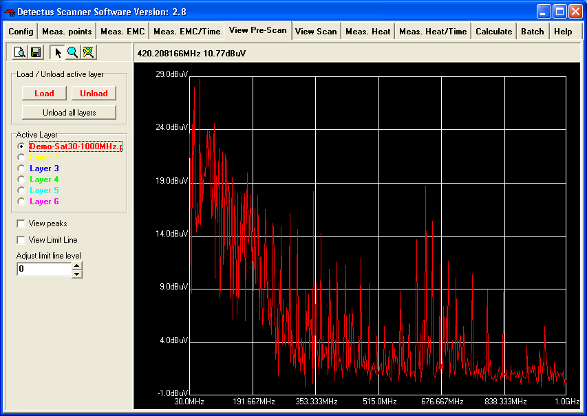
25. Click on the Load button and select the previously saved file.
26. For detailed information on how to operate the View Pre-Scan tab, please refer to table of contents.
27. The result of a Pre-Scan measurement can be documented as a report in HTML format and printed out.
7. How to perform a spot Heat measurement over a period of time (DS and Rx series)
This chapter will guide you step by step through the heat measurement of a spot during a period of time.
1. Start the software by clicking on the icon on your desktop.
2. After a few seconds, this dialog box will show.
3. Click on Yes to reset the Scanner to its starting position at coordinates X0 Y0 Z10.
4. Position and calibrate the IR-probe according to the procedure in “Positional calibration of the IR-probe”.
5. Click on the Meas. Heat/Time tab.
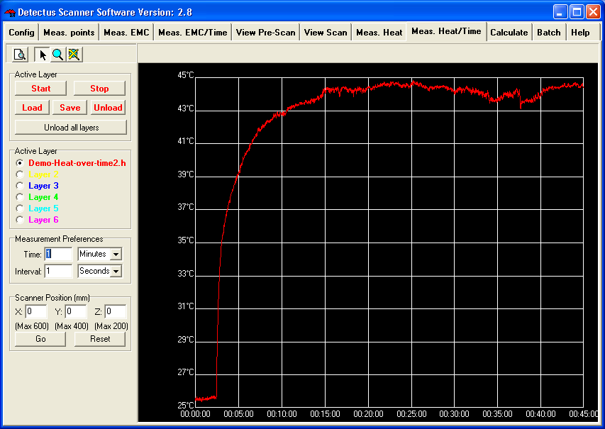
6. Enter the desired coordinates into Scanner Position (mm) box, and click on the Go button to move the Scanner and aim the IR-probe towards the spot to be measured.
7. Verify the position of the IR-probe by pressing the LASER ON button on top of the IR-probe. (The laser will light for approximately 15 seconds.)
8. In Measurement Preferences enter the total measuring time in the Time box.
9. In Measurement Preferences enter the interval desired between the individual measurements in the Interval box.
10. In the Active Layer box, select a colored layer.
11. Start the measurement by clicking on the Start button.
12. When the measurement is finished you can click on the Save button to save the measurement as a .HOT file.
(Saving is optional but you will find it useful when you want to repeat a measurement and compare the results.
8. How to perform a spot EMC measurement over a period of time
This chapter will guide you, step by step, through making a spot EMC measurement over a period of time.
1. Start the software by clicking on the icon on your desktop.
2. After a few seconds, this dialog box will show.
3. Click on Yes to reset the Scanner to its starting position at coordinates X0 Y0 Z10.
4. Position and calibrate the IR-probe according to the procedure in “Positional calibration of the IR-probe”.
5. Click on the Meas. EMC/Time tab.
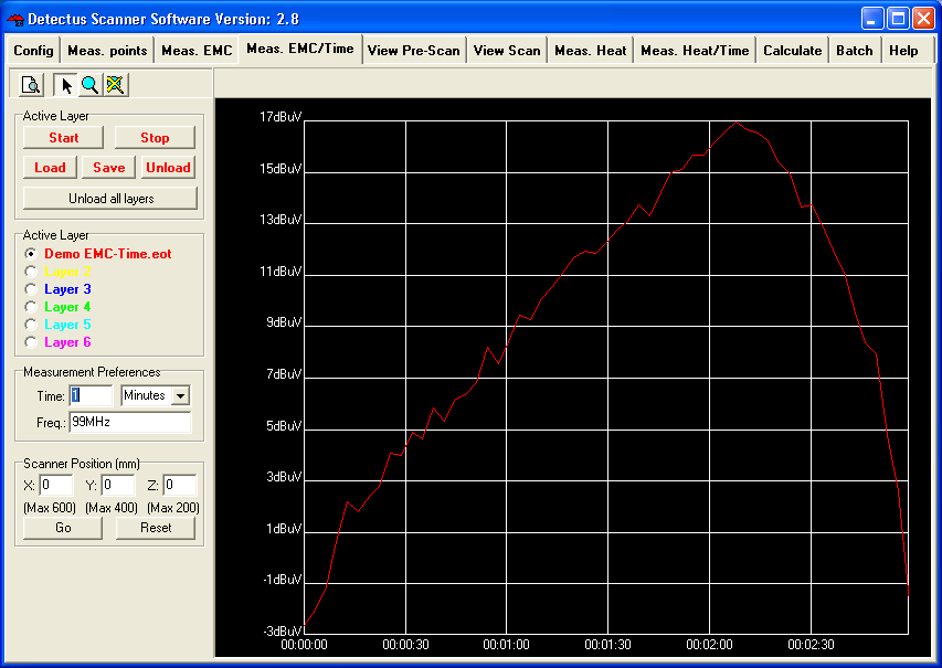
6. Enter the desired coordinates into Scanner Position (mm) box, and click on the Go button to move the Scanner and place the near field probe above the spot you want to measure.
7. In Measurement Preferences enter the total measuring time in the Time box.
8. In Measurement Preferences enter the desired frequency in the Frequency box. Allowed units are Hz, kHz, MHz and GHz.
9. In the Active Layer box, select a colored layer.
10. Start the measurement by clicking on the Start button.
11. When the measurement is finished you can click on the Save button to save the measurement as a .EOT file.
(Saving is optional but you will find it useful when you want to repeat a measurement and compare the results.)
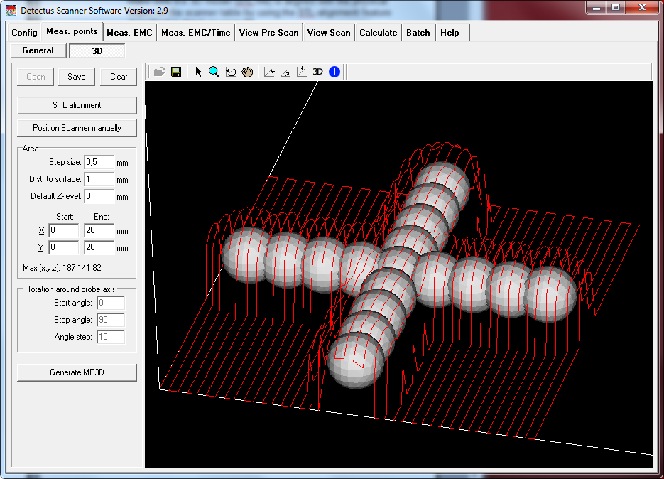
9. How to generate 3D measuring points
3D measuring points are based on a 3D surface model in STL file format.
The measuring points are generated to form an offset surface to the STL file.
1. Click on the Meas. points tab.
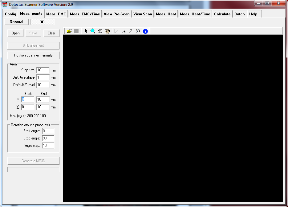
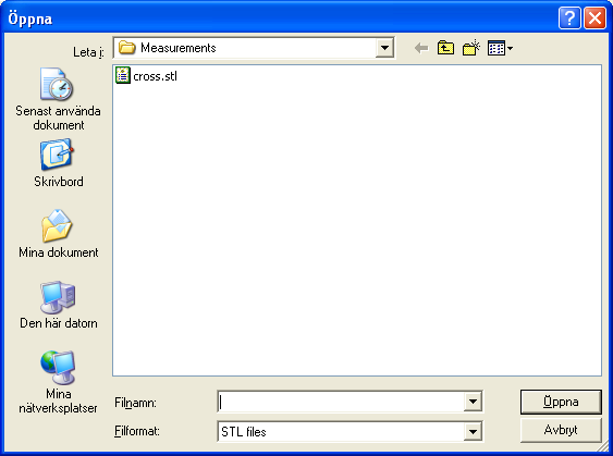
2. Click on the OPEN button to open an STL-file. Both ASCII and Binary STL-files are supported.
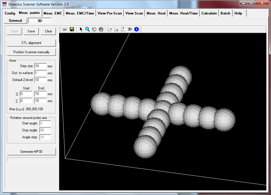
3. The STL-file view can be rotated, zoomed and panned
4. Click on the STL alignment button.
Make sure the 3D model (STL-file) is aligned with the physical object on the scanner table by using the STL-alignment feature described in detail on page 103.
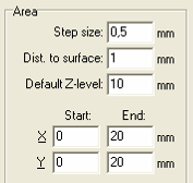
5. Set up the scanning area
6. Click on the Generate MP3D button to generate the measuring points.
Generation may take some time if the 3D model is complex. A blue bar will show the progress.
Generation can be stopped by clicking again on the same button.
10. How to make calculations
On the Calculate tab, you can perform four different calculations based on measurements. The calculations are as follows:
1. Concatenate EMC-Scan measurements is a vector addition, measuring point by measuring point, of two previously saved EMC-Scan measurements. T h i s calculation is intended to eliminate the irregular appearence of the appearance of a measured field, caused by the difference in sensitivity in different angles of a dipole antenna. Perform a measurement, turn the antenna (probe) 90° and perform another measurement, then concatenate the two measurements.
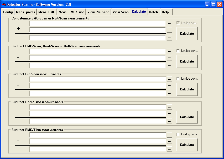
2. Subtract EMC-Scan or Heat-Scan measurements is a subtraction, measuring point by measuring point, of two previously saved EMC-Scan or Heat-Scan measurements. This calculation is intended to visualize the difference between two EMC-Scan or two Heat-Scan measurements. For example, one measurement performed before and one after an alteration to the test object.
3. Subtract Pre-Scan measurements is a subtraction of two previously saved Pre-Scan measurements.
This calculation is intended to visualize the difference between two Pre-Scan measurements. For example, one measurement performed before and one after an alteration to the test object.
4. Subtract Heat/Time measurements is a subtraction of two previously saved Heat/Time measurements.
This calculation is intended to visualize the difference between two Heat/Time measurements. For example, one measurement performed before and one after, an alteration to the test object.
5. Subtract EMC/Time measurements is a subtraction of two previously saved EMC/Time measurements.
This calculation is intended to visualize the difference between two EMC/Time measurements. For example, one measurement performed before and one after an alteration to the test object.
10.1. Lin/Log
Activating Lin/Log means that the calculation is performed in linear mode instead of logarithmic mode.
That is, all values are first converted from logarithmic mode to linear mode then the calculation is performed and then the result of the calculation is converted back to logarithmic mode.
Please note!
A negative linear result cannot be converted to log mode.
To resolve that the minus sign is removed before converting to log mode and then added to the result after conversion.
To make a calculation, do as follows:

Click on the Calculate button to perform the calculation.
The resulting file can now be visualized on the corresponding View tab.